A while ago I had some climate data that I needed to play with, but they were in a “wide” format that made analysis in R difficult. These data were obtained from weather stations across the range of C. xantiana, and their format may make sense to us humans, but for data wrangling / analysis, they’re hard to work with.
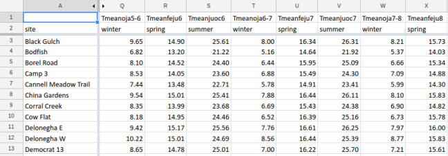
                  site easting Pnoja_2006 Pfeju_2006 Pjuoc_2006 Pnoja_2007 Pfeju_2007 Pjuoc_2007
1          Black Gulch  361558     127.70     152.38      50.90      73.18      76.04       8.64
2              Bodfish  369100     114.59     162.21      56.68      67.22      71.59      13.51
3           Borel Road  362540     120.32     151.20      53.77      76.90      75.32       8.72
4               Camp 3  369107     173.81     168.17      27.83      60.04      64.64       8.63
5 Cannell Meadow Trail  372040     156.40     145.40      24.16     144.50      59.30       9.00
6        China Gardens  350537     132.16     171.44      29.61      99.60     139.60      17.52
The table shows a portion of the nine years of climate data.”Pnoja_2006″ is precipitation received between November 2005 and January 2006, “Pfeju_2006” is precipitation received between February and June 2006 (we’re working with a winter germinating annual, so we’re splitting the climate into early, mid, and late portions of it’s life history). I would have named things differently, but you work with what you’ve got!
We need to reshape the data into “long” format, where each row represents a single year (“year” being used loosely here, in a more biological than calendar sense — November (germination) to June (seed set)). There are many tutorials on using reshape functions in R, but I found many of them unclear, or addressing problems slightly different from my own. I decided to use dplyr and plyr, but you can do all of this with the reshape2 package, as well.
reshape2 digression
The tidyr results below can be obtained in one line of code with reshape in the reshape2 package, like this
climateLong <- reshape(climateWide, varying = c(3:32), dir = "long", idvar = "site", sep = "_", timevar = "year")
I may just be overlooking some tidyr functionality that would make it this easy — if you know how, please let me know! I described the tidyr methods because the grammer is a bit more intuitive and I’m enjoying working with dplyr / tidyr a lot, but don’t know if there’s any good reason to use it (for this kind of problem) instead of reshape.
tidyr code
Here’s the tidyr code, with more explanation beneath. You can download a test data set here.
# load packages
library(tidyr)
library(plyr)

# read in messy, wide data file
climateWide <- read.csv("Downloads/Climate.csv", header = T, sep = ',')

# use gather to go from wide to long format, then separate year and season, then spread seasons back across columns
climateLong <- climateWide %>% gather(key, value, -site, -easting) %>%
separate(key, into = c("season", "year"), sep = "_") %>%
spread(season, value) %>%
rename(c("Pnoja" = "WinterPrecip", "Pfeju" = "SpringPrecip", "Pjuoc" = "SummerPrecip"))
Stepping through the functions:
- gather takes the wide df, climateWide, and flips it to long-form. First you choose a column name for the ‘key’ — the variable you’re flipping long-ways, here ‘Pnoja_2006’, ‘Pfeju_2006’, etc. — I just used ‘key’. ‘Value’ in this case is the observed precipitation; you can name it ‘precip’ or whatever. We also need to specify the variables we don’t want gathered — here, site and easting — these will be copied down in the new rows with their appropriate keys and values. All other columns will be gathered. (The ‘pipe’, %>%, in this code allows us to simply pass the dataframe between functions without having to name the df explicitly)
- separate is needed to split the ‘key’ (e.g., Pfeju_2006) into season and year. We just tell it what the key is (easy in this case), what we want to name our new variables we’re splitting the key into (‘season’ and ‘year), and what separates the variables in the key (here, ‘_’).
- I need to use spread because for my purposes, this data set is now a bit too long. Each seasonal precipitation observation is on a separate row (ie, there are three rows for each year) — for the analysis I’m doing, I need each row to refer to a single year. So we use the opposite of gather, spread, to bring the ‘season’ key out of long into wide format, and supply the value associated with it (‘value’).
- Then we just use rename to give our seasonal precipitation variables clearer names.
We end up with:
          site easting year WinterPrecip SpringPrecip SummerPrecip
1  Black Gulch  361558 2006       127.70       152.38        50.90
2  Black Gulch  361558 2007        73.18        76.04         8.64
3  Black Gulch  361558 2008       108.97       107.07         4.75
4  Black Gulch  361558 2009       125.88        78.14         7.61
5  Black Gulch  361558 2010       164.73       111.38        30.06
6  Black Gulch  361558 2011       382.49       113.21        25.99
7  Black Gulch  361558 2012        76.50        94.15         9.43
8  Black Gulch  361558 2013        63.90        45.97        32.36
9  Black Gulch  361558 2014        68.49        94.77         8.48
10 Black Gulch  361558 2015       115.13        72.37           NA
11     Bodfish  369100 2006       114.59       162.21        56.68
12     Bodfish  369100 2007        67.22        71.59        13.51
...
Hopefully this all makes sense, and can help somebody get their data set ready for analysis.
